Cross entropy and KL divergence

Posted Jan 31, 2025 Updated Feb 1, 2025

By 信雄湊

14 min read

1. Definitions

KL divergence: $KL(P || Q) = ∑_i P(i) log \bigg[\frac{P(i)}{Q(i)}\bigg]$

Cross entropy: $H(P, Q) = - ∑_i P(i) log [Q(i)]$

The relationship between KL divergence and cross entropy can be expressed as:

\[KL(P || Q) = H(P, Q) - H(P)\]

Where H(P, Q) is the cross entropy between distributions P and Q, and H(P) is the entropy of distribution P.

This formula shows that KL divergence is the difference between the cross entropy of P and Q, and the entropy of P. In other words, KL divergence can be thought of as a correction term added to cross entropy to account for the fact that Q may not perfectly match P. When Q perfectly matches P, the cross entropy is equal to the entropy of P, and the KL divergence is zero. When Q is very different from P, the cross entropy will be much larger than the entropy of P, and the KL divergence will be positive and large.

So, while both KL divergence and cross entropy measure the difference between probability distributions, they have different interpretations and applications, with KL divergence being used more generally and cross entropy being used in the specific context of classification.

What is Cross Entropy?

Cross entropy is a measure of how different two probability distributions are. In the context of machine learning and classification, it is often used to measure the difference between a true probability distribution and a predicted probability distribution.

Imagine that you have a set of data points that belong to one of several classes. The true probability distribution for these classes would give the probability of a data point belonging to each class. If you have a classifier that predicts the probability of a data point belonging to each class, this predicted probability distribution can be compared to the true probability distribution using cross entropy.

The cross entropy between the true probability distribution and the predicted probability distribution is a measure of how well the predicted distribution matches the true distribution. If the predicted distribution is exactly the same as the true distribution, the cross entropy is zero. If the predicted distribution is very different from the true distribution, the cross entropy will be larger.

In machine learning, cross entropy is often used as a loss function during training. The goal is to minimize the cross entropy between the predicted probability distribution and the true probability distribution. This is done by adjusting the parameters of the classifier during training to improve the accuracy of the predictions.

Overall, cross entropy is a useful tool for measuring the difference between two probability distributions, and is particularly important in the context of classification and machine learning.

\[H(P, Q) = - ∑_i P(i) log [Q(i)]\]

where P and Q are probability distributions over the same set of events, and P(i) and Q(i) are the probabilities of the ith event in the distributions.

Let’s break down the formula:

$H(P,Q)$: This is the cross entropy between P and Q, which measures how different Q is from P.
$-∑_i$: This is the summation operator, which means that we are summing over all events i in the distributions.
$P(i)$: This is the probability of the ith event in the true distribution P.
$Q(i)$: This represents the predicted probability distribution of the ith event. In classification problems, Q(i) is often the output of the softmax function, which converts the logits (raw outputs of the model) into a probability distribution.
$log [Q(i)]$: This is the natural logarithm of the predicted probability of the ith event. ==It is used to put more weight on events with low probability, as the logarithm of a value between 0 and 1 is negative and decreases rapidly as the value approaches 0.==
$-∑_i P(i) log [Q(i)]$: This term calculates the average amount of information needed to represent events in P using the probabilities in Q.

The intuition behind this formula is that the cross entropy between P and Q is a measure of how much additional information is needed to represent events in P using the predicted probabilities in Q. When the predicted probabilities are very close to the true probabilities, the cross entropy is small, but when they are very different, the cross entropy is large.

In machine learning, cross entropy is often used as a loss function for training classifiers. The goal is to minimize the cross entropy between the true probability distribution (i.e., the ground truth labels) and the predicted probability distribution output by the model. This is done by adjusting the model’s parameters during training to improve its accuracy in predicting the correct labels.

What is KL divergence?

KL divergence, also known as Kullback-Leibler divergence, is a measure of how different two probability distributions are. In the context of machine learning, it is often used to measure the difference between a predicted probability distribution and a true probability distribution.

The KL divergence between two probability distributions P and Q is defined as follows:

\[D_{KL}(P || Q) = ∑_i P(i) log \bigg[\frac{P(i)}{Q(i)}\bigg]\]

where P and Q are probability distributions over the same set of events, and P(i) and Q(i) are the probabilities of the ith event in the distributions.

Let’s break down the formula:

$D_{KL}(P \vert\vert Q)$: This is the KL divergence between P and Q, which measures how different Q is from P.
$∑_i$: This is the summation operator, which means that we are summing over all events i in the distributions.
$P(i)$: This is the probability of the ith event in the true distribution P.
$log \bigg[\frac{P(i)}{Q(i)}\bigg]$: This is the natural logarithm of the ratio of the probability of the ith event in the true distribution P to the probability of the same event in the predicted distribution Q.

The intuition behind KL divergence is that it measures how much additional information is needed to represent events in P using the probabilities in Q. When P and Q are the same distribution, the KL divergence is zero. When they are different, the KL divergence is greater than zero.

In machine learning, KL divergence is often used as a loss function during training. The goal is to minimize the KL divergence between the predicted probability distribution and the true probability distribution. This is done by adjusting the parameters of the model during training to improve the accuracy of the predictions.

One common application of KL divergence in machine learning is in the training of generative models, such as variational autoencoders (VAEs). In this context, the KL divergence is used to measure the difference between the learned latent space distribution and a prior distribution, such as a Gaussian distribution. By minimizing the KL divergence, the generative model can learn to generate samples that are similar to those in the training data, while also ensuring that the learned latent space has desirable properties, such as smoothness and continuity.

Why Cross Entropy is Negative.

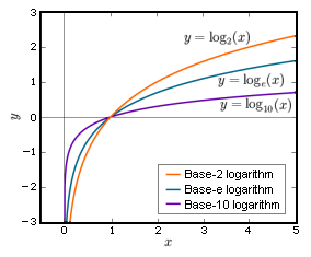
For any base b > 1 logarithms of numbers between 0 and 1 are negative numbers, the logarithm of 1 is 0, and logarithms of numbers greater than 1 are positive real numbers as seen in the image below.

\[H(P, Q) = - ∑_i P(i) log [Q(i)]\]

We often want to measure the performance of a Machine Learning model by its loss function which “Cross Entropy” is almost always the best candidate, sicne the $log[Q(i)]$ and if $Q(i)$ falls into the interval between 0 and 1, the result will become a negative value, and when we use Cross Entropy as a loss function, a positive value is more likely to be measured and huma-readable.

Cross-entropy loss and Kullback-Leibler (KL) divergence are both commonly used loss functions in machine learning. They have a relationship in the sense that KL divergence can be used to measure the difference or “distance” between two probability distributions, and cross-entropy loss can be seen as a special case of KL divergence.

Cross-entropy loss is primarily used for classification tasks and measures the dissimilarity between the predicted probability distribution and the true distribution (one-hot encoded labels). It calculates the average negative log-likelihood of the predicted probabilities for the correct class. Cross-entropy loss is defined as:

\[H(p, q) = - ∑ p(x) * log(q(x))\]

where p(x) represents the true distribution (one-hot encoded labels) and q(x) represents the predicted distribution (softmax output probabilities).

On the other hand, KL divergence is a measure of the difference between two probability distributions. It quantifies how much one distribution differs from the other. KL divergence is defined as:

\[D_KL(p || q) = ∑ p(x) * log(p(x) / q(x))\]

In the context of knowledge distillation, where we have soft targets (teacher model’s output probabilities) and hard targets (one-hot encoded labels), KL divergence is used to measure the difference between the soft targets and the student model’s predictions. By minimizing the KL divergence, the student model learns to mimic the soft targets generated by the teacher model.

It’s worth noting that when the true distribution p(x) is a one-hot encoded label (i.e., a discrete distribution), the KL divergence simplifies to the cross-entropy loss. Therefore, cross-entropy loss can be seen as a special case of KL divergence where the true distribution is a one-hot encoded label.

In summary, cross-entropy loss is a specific form of KL divergence, where the true distribution is a one-hot encoded label. In knowledge distillation, KL divergence is used to compare the soft targets and the student model’s predictions, allowing the student model to learn from the more refined information provided by the teacher model.

2. Entropy explained

The entropy formula quantifies the amount of uncertainty or randomness in a probability distribution. It is a foundational concept in information theory introduced by Claude Shannon.

For a discrete random variable $X$ with possible outcomes $x_1, x_2, \dots, x_n$ and a probability mass function $P(X = x_i) = p_i$, the entropy $H(X)$ is defined as:

\[H(X) = -\sum_{i=1}^{n} p_i \log p_i,\]

where

$H(X)$: The entropy of the random variable $X$.
$p_i$: The probability of the $i$-th outcome ($0 \leq p_i \leq 1$).
$\log$: The logarithm function (base 2 is common in information theory, while base $e$ is used in other contexts like physics).

Key Properties

Non-Negativity:
- $H(X) \geq 0$. Entropy is always non-negative.
- $H(X) = 0$ if and only if one outcome has a probability of $1$ (no uncertainty).
Maximum Entropy:
- Entropy is maximized when all outcomes are equally likely ($p_i = \frac{1}{n}$): $H_{\text{max}} = \log n$
Unit of Measurement:
- If the logarithm is base $2$, entropy is measured in bits.
- If the logarithm is base $e$, entropy is measured in nats.

3. Entropy for Continuous Random Variables**

For a continuous random variable $X$ with probability density function $f(x)$, the differential entropy is given by:

\[H(X) = -\int f(x) \log f(x) \, dx\]

4. Example Calculations

Case 1: A Fair Coin A fair coin has two outcomes ($n = 2$) with equal probabilities $p_1 = p_2 = 0.5$. Entropy is:

\[H(X) = -\sum_{i=1}^{2} p_i \log_2 p_i = -\left(0.5 \log_2 0.5 + 0.5 \log_2 0.5\right)\]

Since $\log_2 0.5 = -1$: $H(X) = -\left(0.5 \times -1 + 0.5 \times -1\right) = 1 \, \text{bit}$

Case 2: A Biased Coin A biased coin with $p(\text{Heads}) = 0.8$ and $p(\text{Tails}) = 0.2$:

\[H(X) = -\left(0.8 \log_2 0.8 + 0.2 \log_2 0.2\right)\]

Approximating values: $\log_2 0.8 \approx -0.3219, \quad \log_2 0.2 \approx -2.3219$ $H(X) \approx -\left(0.8 \times -0.3219 + 0.2 \times -2.3219\right) \approx 0.7219 \, \text{bits}$

5. Applications of Entropy

Information Theory:
- Measures the uncertainty in a source.
- Basis for concepts like mutual information and Kullback-Leibler divergence.
Data Compression:
- Entropy sets a theoretical limit for lossless data compression.
Machine Learning:
- Used in loss functions like cross-entropy.
- Helps quantify uncertainty in probability distributions (e.g., predictive models).
Physics and Thermodynamics:
- Measures disorder or randomness in systems.

6. Why do we use logarithm in the computation of entropy?

The use of the logarithm in measuring information content and defining entropy has deep theoretical and practical justifications. Here’s why the logarithmic function is specifically chosen:

Logarithm Captures the Nature of Information

The information content (or “surprise”) of an event is inversely proportional to its probability. The less likely an event is, the more surprising it is when it occurs. The logarithmic function satisfies this property in a way that aligns with our intuitive and mathematical understanding:

Proportionality to Inverse Probability
For an event with probability $p_i$, the information content is $-\log(p_i)$. This grows as $p_i$ becomes smaller.
- Example:
  - If $p = 0.1$, $-\log(0.1) \approx 2.3$.
  - If $p = 0.01$, $-\log(0.01) \approx 4.6$.
This means rare events (low $p$) provide exponentially more information, which reflects how “surprising” they are.

Logarithms Make Information Additive

One of the most compelling reasons for using logarithms is their property of additivity. This is critical when dealing with independent events.

Additivity Example:

Suppose we observe two independent events $A$ and $B$, with probabilities $p_A$ and $p_B$. The combined probability is $p_A \cdot p_B$.
The total information content of both events is: $I(A, B) = -\log(p_A \cdot p_B) = -\log(p_A) - \log(p_B)$
This additivity is consistent with how we naturally think of combining independent pieces of information.

Without logarithms, we would lose this convenient property.

Exponential Growth of Surprise Logarithms provide a natural way to represent the exponential nature of probability changes in terms of information content.

Example: If an event becomes 10x less likely:

The surprise increases by an additive constant: $I = -\log(p) \quad \text{and if } p' = \frac{p}{10}, \quad I' = -\log(p') = -\log(p) + \log(10)$

This aligns with intuition: Rare events (smaller probabilities) contribute disproportionately more to the uncertainty of a system.

Logarithms Align with Human Perception

Humans perceive many phenomena on a logarithmic scale:

Sound intensity: Measured in decibels (logarithmic scale).
Brightness: Perceived logarithmically.
Information: Intuitively, the difference between probabilities $0.1$ and $0.01$ feels much larger than between $0.9$ and $0.8$.

The logarithmic relationship aligns well with our perception of surprise or information.

Optimal Encoding in Information Theory

In information theory, the logarithmic function ensures that entropy reflects the optimal length of encoding data:

The average number of bits required to encode an event optimally is proportional to $-\log(p_i)$.
Shannon’s entropy provides the theoretical limit for data compression. Without logarithms, this connection would break.

Base of the Logarithm The choice of the logarithm base depends on the context:
Base 2 ($\log_2$): Used in information theory; measures information in bits.
Base e ($\ln$): Common in mathematics and physics; results in information measured in nats.
Base 10 ($\log_{10}$): Sometimes used for interpretability in real-world applications.

Regardless of the base, the properties of the logarithm (proportionality, additivity, and exponential scaling) hold.

Alternative Functions? Why not use a different function (e.g., linear or polynomial)?
A linear function (e.g., $-p_i$) doesn’t capture the exponential growth of surprise for rare events.
A polynomial function doesn’t provide the additive property for independent events.

Logarithms are the unique function that satisfies all the requirements for measuring information content:

Proportional to inverse probability.
Additive for independent events.
Aligns with exponential scaling.

7. Summary

Logarithms are used in entropy and information content because they:

Capture the intuitive relationship between probability and surprise.
Provide additivity for independent events.
Reflect the exponential growth of surprise as probability decreases.
Align with human perception and optimal encoding in information theory.

Data Science

Math

This post is licensed under CC BY 4.0 by the author.